This week I got a task to randomly generate pairs based on a name list. After googling on the internet, I found a perfect solution to achieve my goal.
Here are the detailed steps to achieve a random pair of two, and it’s easy to adjust to your specific needs.
All the example data and formula can be found in this Google Sheet: Random Pairs .
Steps
Step 1 - Generate random numbers using RAND()
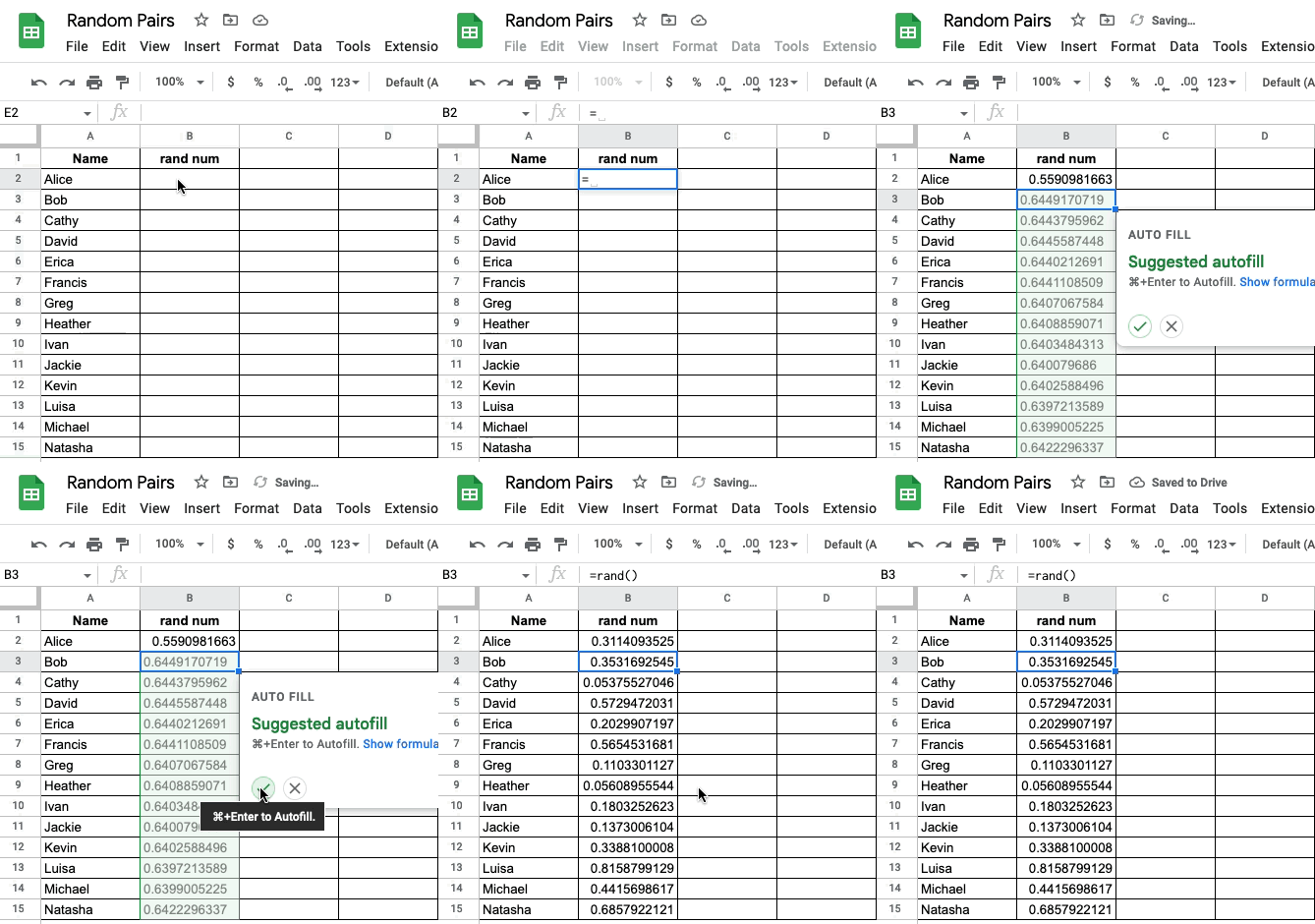
Firstly, we need to generate a random number against each name, we can use the RAND() function to achieve that.
| |

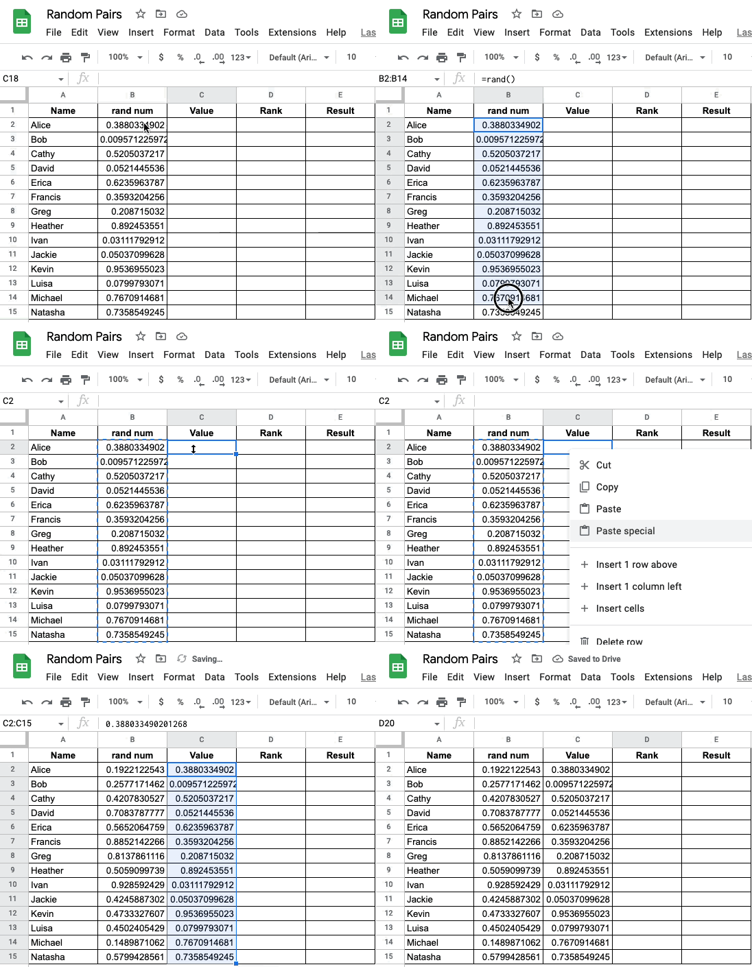
Step 2 - Copy the random number values to a new column named Value
Every time when you hit the Save button in Excel or Google Sheets, it will automatically re-generate a new series of random numbers with the RAND() function. This is not ideally because we want to have a static random number for each person so that we can calculate their rank later on.
An easy solution is to just create a new column, and only copy these random values there in the new column to get these static numbers.

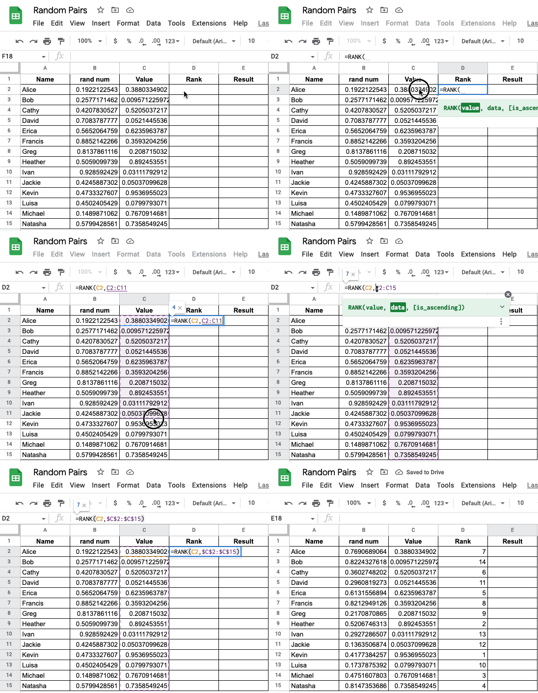
Step 3 - Create ranking on column with RANK()
When we use the RANK() function, one thing needs to be careful is to put the $ sign to lock the data section that you will use in the RANK() function.
| |

Step 4 - Pair up people with CEILING()
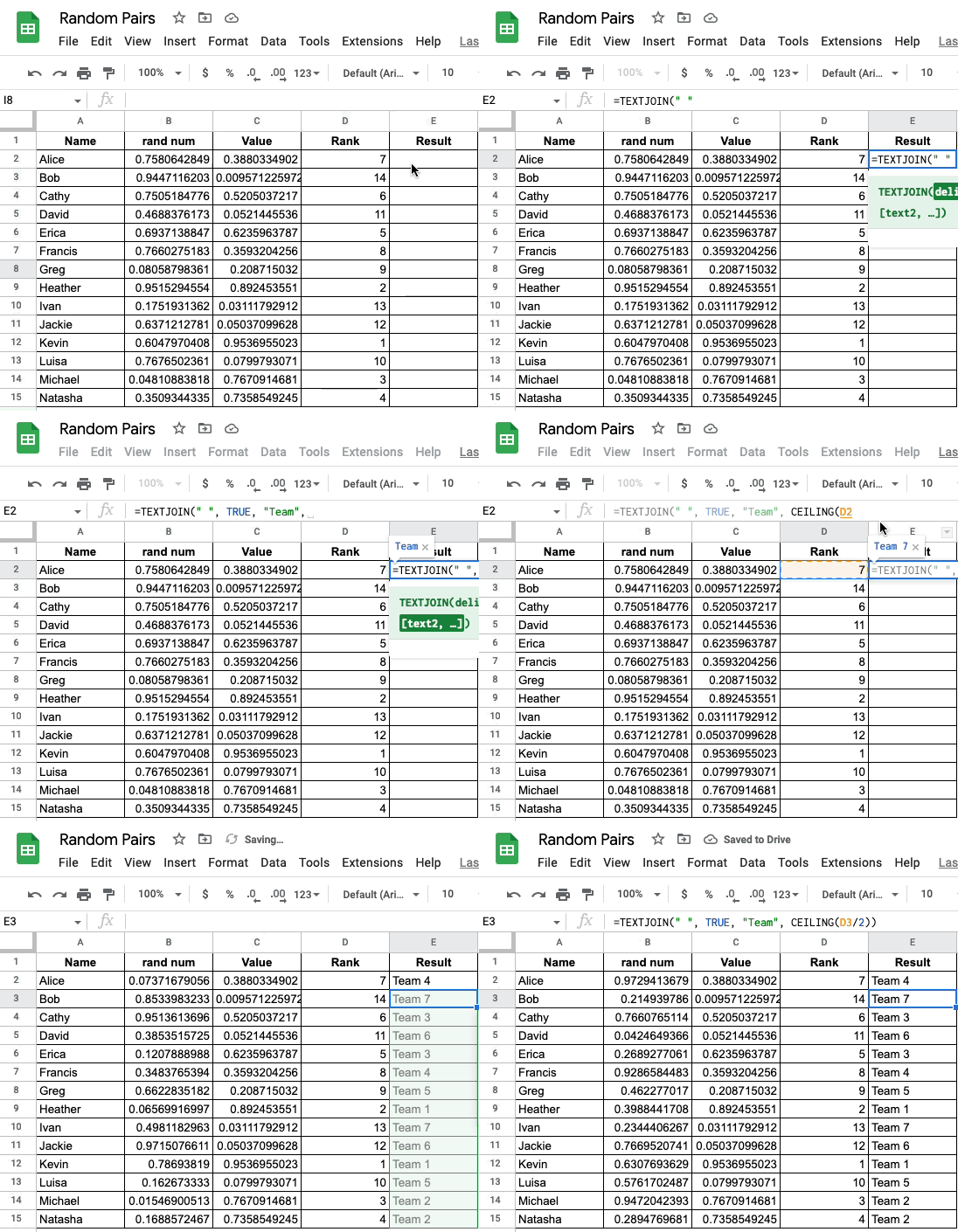
Here we use a formula combination of TEXTJOIN() and CEILING() to create the random pair, with the following excel formula
| |
Here CEILING(D2/2) function will help you to pair up two person as your expected group, and the TEXTJOIN() function is just to concatenate the result ‘Team 1’ string.
If you need to create a random pair of three, you just need to change the CEILING() function to CEILING(D2/3).

Hope it helps.